Complex plane plots in Plots
The plots below are made using the defaults
update_theme!(linewidth=3, Axis=(autolimitaspect=1,))Point-based plots for complex vectors
A vector of complex-typed values will be interpreted as specifying points using the real and imaginary parts.
using ComplexPlots, CairoMakie
z = [complex(cospi(t), 0.4sinpi(t)) for t in (0:400)/200]
lines(z)
scatter!(1 ./ z, marker=:circle, markersize=8, color=:black)
Use sphereplot to make plots on the Riemann sphere.
sphereplot(z, markersize=5)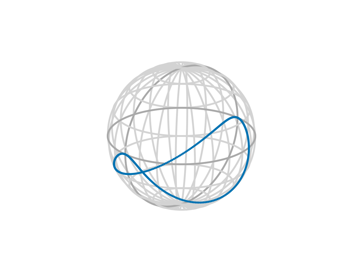
ComplexPlots.sphereplot — Functionsphereplot(z; kw...)Plot a vector of complex numbers on the Riemann sphere. Keyword arguments are:
sphere:falseto disable the sphere, or a tuple(nlat, nlon)to set the number of latitude and longitude lines.markersize: size of the markersline:trueto connect the markers with lines
Function visualization
Plots of complex functions can be made using the zplot function. At each point in the complex domain, the hue is selected from a cyclic colormap using the phase of the function value, and the color value (similar to lightness) is chosen by the fractional part of the log of the function value's magnitude.
Examples:
zplot(z -> (z^3 - 1) / (3im - z)^2)
As you see above, zeros and poles occur where the contours of magnitude collapse into a point. Zeros are characterized by a clockwise progression of the hues green–yellow–magenta–blue around that point, whereas poles have those hues in counterclockwise order. The number of times these hues cycle around the point is the multiplicity of the zero or pole.
zplot(tanh, [-5, 5], [-5, 5])
Above you can see poles and zeros alternating on the imaginary axis.
zplot(z -> log((1 + z) / (1im - z)), [-2, 2], [-2, 2], 1000)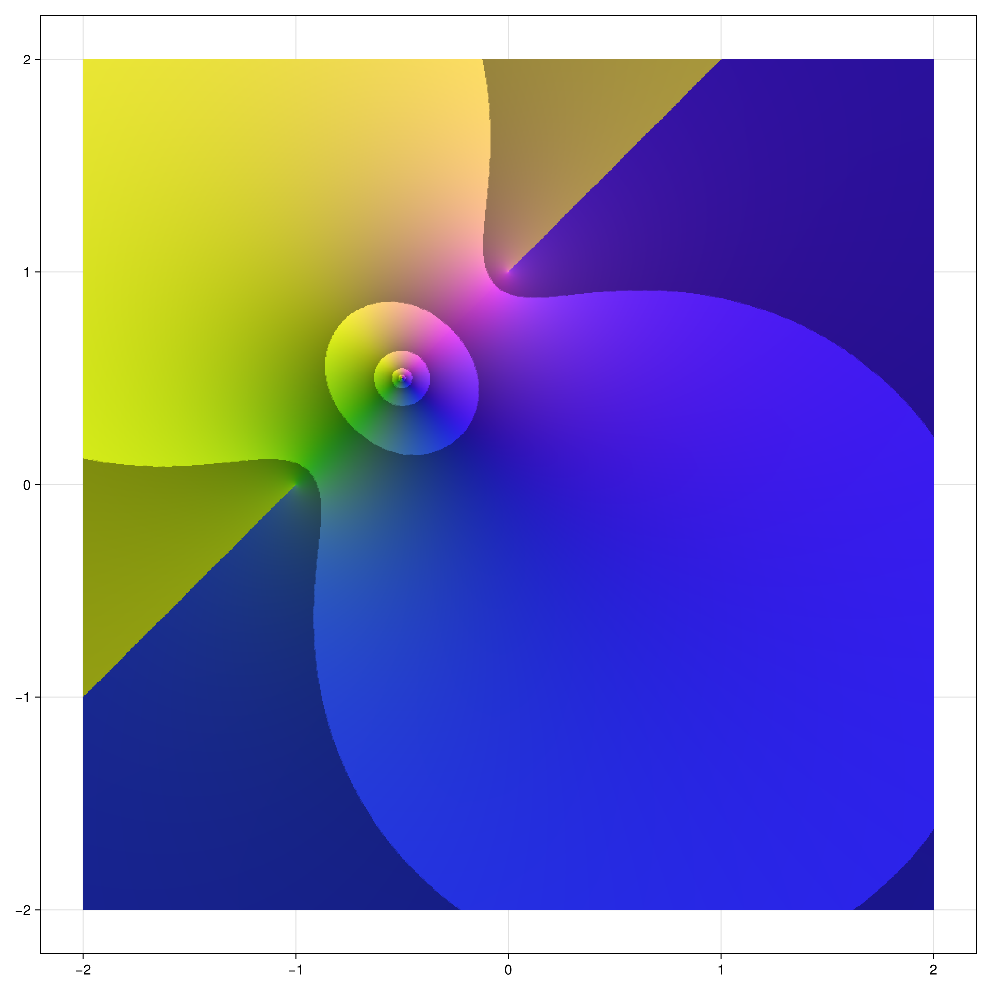
Above you see how branch cuts create abrupt changes in hue. (The final positional argument in the call specifies the number of points used in each direction.)
If you want to plot over a non-rectangular domain, use NaN to indicate points outside the domain:
z = [complex(x,y) for x in range(-1.1, 1.1, 800), y in range(-1.1, 1.1, 800) ]
z[@. abs(z) > 1] .= NaN
log2_artist = artist(2)
zplot( real(z), imag(z), @. (1-z)/(1+z); coloring=log2_artist)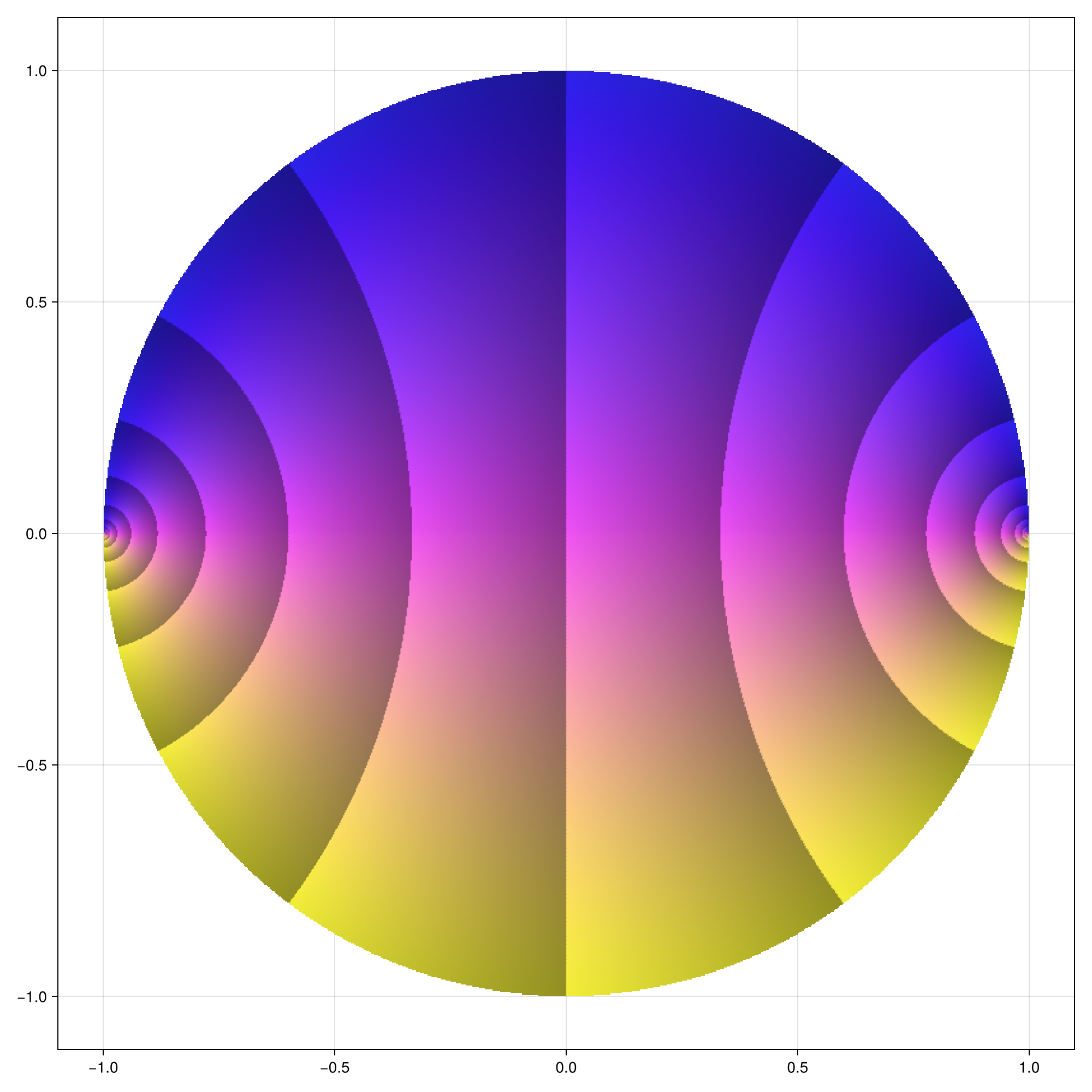
Curves and paths
The ComplexRegions package defines types for lines, circles, rays, segments, and arcs.
Because Makie has its own definitions for Circle and Arc, you must either qualify the names or specify the unqualified versions as follows:
using ComplexRegions
const Circle = ComplexRegions.Circle;
const Arc = ComplexRegions.Arc;ComplexRegions.Arcplot(Circle(-1, 1))
lines!(Segment(-1-1im, -1+1im))
scatter!(Arc(-1, 1im, 1), color=:darkred)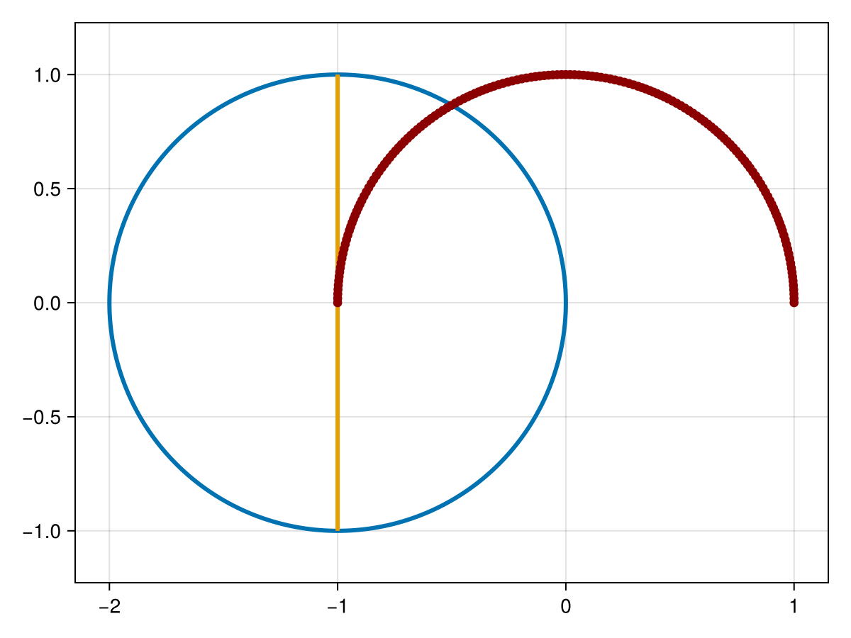
You can also create and plot polygons.
L = Polygon([0, 1im, -1+1im, -1-1im, 1-1im, 1])
plot(L)  # or poly(L) for filled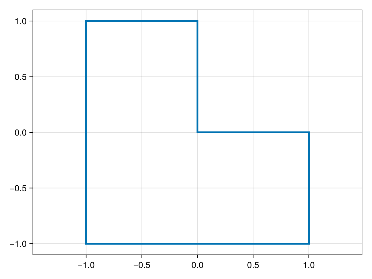
There are some predefined shapes in the Shapes submodule.
lines(Shapes.ellipse(1, 0.5))
lines!.([
    2im + Shapes.star,
    -2im + Shapes.cross,
    2 + Shapes.triangle,
    -2 + 0.3im*Shapes.hypo(3)
    ])
Regions
The ComplexRegions package defines types for regions, which are interior and/or exterior to closed curves and paths.
C = Circle(0, 1);  S = Shapes.square;
fig = Figure()
ax = [Axis(fig[i,j]) for i in 1:2, j in 1:2]
poly!(fig[1,1], interior(C))
poly!(fig[1,2], exterior(S))
ax[1,2].limits[] = (-3, 3, -3, 3)
poly!(fig[2,1], between(2C, S))
poly!(fig[2,2], ExteriorRegion([C - 2, S + 2]))
ax[2,2].limits[] = (-3, 3, -3, 3)