Comparison to AAA in SciPy

The SciPy library includes an implementation of the AAA algorithm for rational approximation in its scipy.interpolate module. Below is a comparison of pyratapprox’s AAA and Thiele continued fraction methods against SciPy’s AAA implementation.

Timing

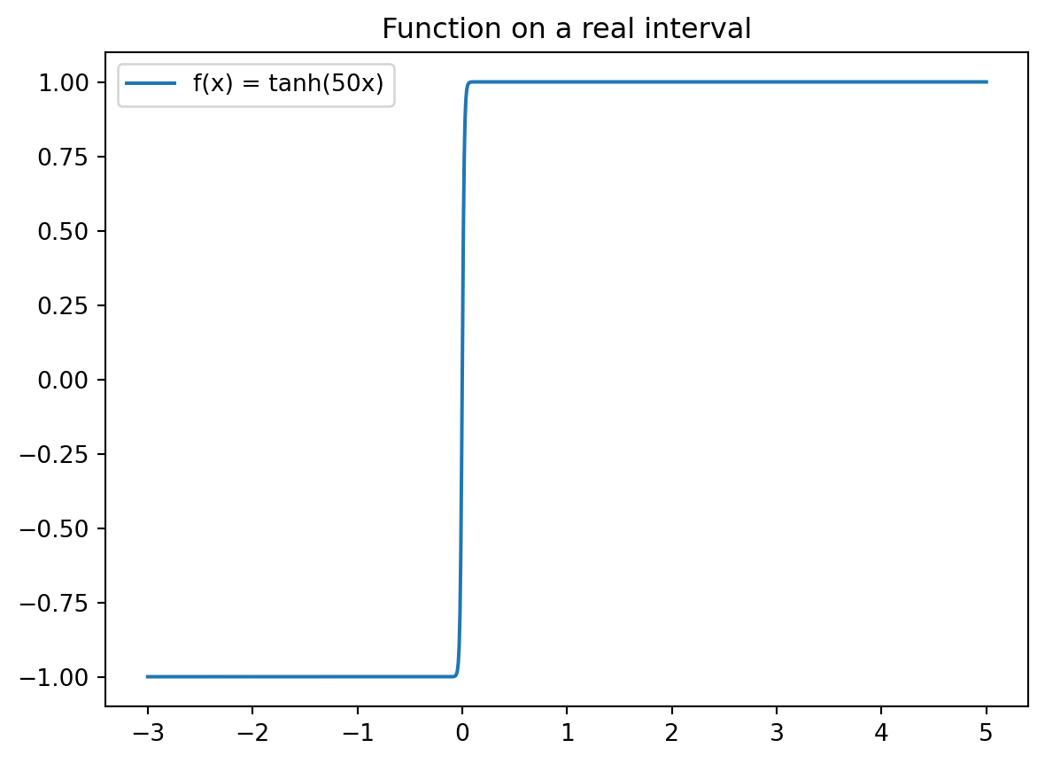
from pyratapprox import *
import numpy as np
from scipy.interpolate import AAA as spAAA
import matplotlib.pyplot as plt

x = np.linspace(-3, 5, 1000)
f = np.tanh(50 * x)
plt.plot(x, f, label='f(x) = tanh(50x)')
plt.title('Function on a real interval')
plt.legend();

Detected IPython. Loading juliacall extension. See https://juliapy.github.io/PythonCall.jl/stable/compat/#IPython

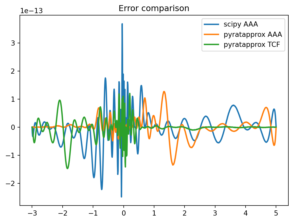
Here, we generate rational approximations using all three methods:

r_scipy = spAAA(x, f)
r_aaa = approximate(f, x, method=AAA)
r_tcf = approximate(f, x, method=TCF)
print("Degrees:")
d = len(r_scipy.support_points) - 1
print(f"scipy AAA:       ({d}, {d})")
print(f"pyratapprox AAA: {r_aaa.degrees()}")
print(f"pyratapprox TCF: {r_tcf.degrees()}")

Degrees:
scipy AAA:       (31, 31)
pyratapprox AAA: (32, 32)
pyratapprox TCF: (32, 32)

As you see above, the results of the three methods are nearly identical in terms of the resulting rational type. Both of the AAA results use essentially the same algorithm, while TCF uses an algorithm that is asymptotically faster. The errors are all similar:

fig, ax = plt.subplots()
test_pts = np.linspace(-3, 5, 1000)
ax.plot(test_pts, np.tanh(50 * test_pts) - r_scipy(test_pts), '-', label='scipy AAA', lw=2)
ax.plot(test_pts, np.tanh(50 * test_pts) - r_aaa(test_pts), '-', label='pyratapprox AAA', lw=2)
ax.plot(test_pts, np.tanh(50 * test_pts) - r_tcf(test_pts), '-', label='pyratapprox TCF', lw=2)
ax.legend()
ax.set_title('Error comparison');

When the rational degree exceeds about 20, the pyratapprox methods are significantly faster to build than SciPy’s AAA implementation, as shown below:

import timeit
n = 50
time_scipy = timeit.timeit('spAAA(x, f)', globals=globals(), number=n) / n
time_aaa = timeit.timeit('approximate(f, x, method=AAA)', globals=globals(), number=n) / n
time_tcf = timeit.timeit('approximate(f, x, method=TCF)', globals=globals(), number=n) / n
print(f"Average build time over {n} runs:")
print(f"scipy AAA: {time_scipy*1e3:.2f} milliseconds")
print(f"pyratapprox AAA: {time_aaa*1e3:.2f} milliseconds")
print(f"pyratapprox TCF: {time_tcf*1e3:.2f} milliseconds")

Average build time over 50 runs:
scipy AAA: 34.35 milliseconds
pyratapprox AAA: 11.40 milliseconds
pyratapprox TCF: 7.80 milliseconds

Evaluation times also favor pyratapprox:

n = 200
time_scipy = timeit.timeit('r_scipy(test_pts)', globals=globals(), number=n) / n
time_aaa = timeit.timeit('r_aaa(test_pts)', globals=globals(), number=n) / n
time_tcf = timeit.timeit('r_tcf(test_pts)', globals=globals(), number=n) / n
print(f"Average evaluation time over {n} runs:")
print(f"scipy AAA: {time_scipy*1e6:.2f} microseconds")
print(f"pyratapprox AAA: {time_aaa*1e6:.2f} microseconds")
print(f"pyratapprox TCF: {time_tcf*1e6:.2f} microseconds")

Average evaluation time over 200 runs:
scipy AAA: 132.04 microseconds
pyratapprox AAA: 109.33 microseconds
pyratapprox TCF: 84.56 microseconds

Approximation in continuous mode

In addition, pyratapprox offers automatic refinement of the domain discretization, which can safeguard against accuracy loss when singularities are present near the domain. For example, consider approximation on the unit circle of the function \(f(z) = \sqrt{1.001 + z}\). If we use 400 points in SciPy’s AAA, everything seems OK:

z = np.exp(1j * np.pi * np.linspace(-1, 1, 200))
f = np.sqrt(1.001 + z)
r = spAAA(z, f)
print(f"In scipy AAA, degree {len(r.support_points) - 1} achieves estimated accuracy {r.errors[-1]:.2e}")

In scipy AAA, degree 17 achieves estimated accuracy 2.79e-13

However, if we look more closely near the branch point at \(z = -1.001\), we see that the domain is badly under-resolved:

test_pts = np.exp(1j * np.pi * np.linspace(-1, 1, 5000))
test_f = np.sqrt(1.001 + test_pts)
print(f"Max observed error on 5000 points: {np.max(np.abs(test_f - r(test_pts))):.2e}")

Max observed error on 5000 points: 1.93e-04

By approximating on the unitcircle domain without prior discretization, the algorithm automatically refines the point set to achieve the advertised accuracy:

f = lambda z: np.sqrt(1.001 + z)
r = approximate(f, unitcircle)    # AAA is the default method
max_err = np.max(np.abs(test_f - r(test_pts)))
print(f"In pyratapprox AAA, degree {r.degree()} achieves max observed error {max_err:.2e}")

In pyratapprox AAA, degree 27 achieves max observed error 3.10e-13