Algorithms

There are three algorithms for rational approximation offered in this version of the package:

AAA : Adaptive iteration based on the barycentric representation of rational functions [1], [2].

Thiele continued fractions : Adaptive iteration based on the Thiele continued fraction representation of rational functions [5].

Partial fractions with prescribed poles : Linear least-squares approximation with user-specified poles [4].

The first two algorithms are nonlinear but capable of high accuracy with automatic selection of poles. The third algorithm is linear and fast, but achieving high accuracy depends on the singularity structure and the quality of information known about it.

Each algorithm has a discrete variant, which approximates values given on a point set, and a continuum variant, which approximates a function defined on a piecewise-smooth domain in the complex plane. The continuum variants are generally more robust and accurate when there are singularities near the domain of approximation.

AAA algorithm

using RationalFunctionApproximation, CairoMakie

The AAA algorithm is the best-known and most widely used method for rational approximation. Briefly speaking, the AAA algorithm maintains a set of interpolation nodes (called support points in the AAA literature) and a set of sample points on the boundary of the domain. The node set is grown iteratively by finding the best approximation in a least-squares sense on the sample points using the interpolation nodes, then greedily adding the worst-case sample point to the node set.

The convergenceplot function shows the errors of the approximants found during the AAA iteration.

f = x -> cos(exp(3x))
r = approximate(f, unit_interval)
convergenceplot(r)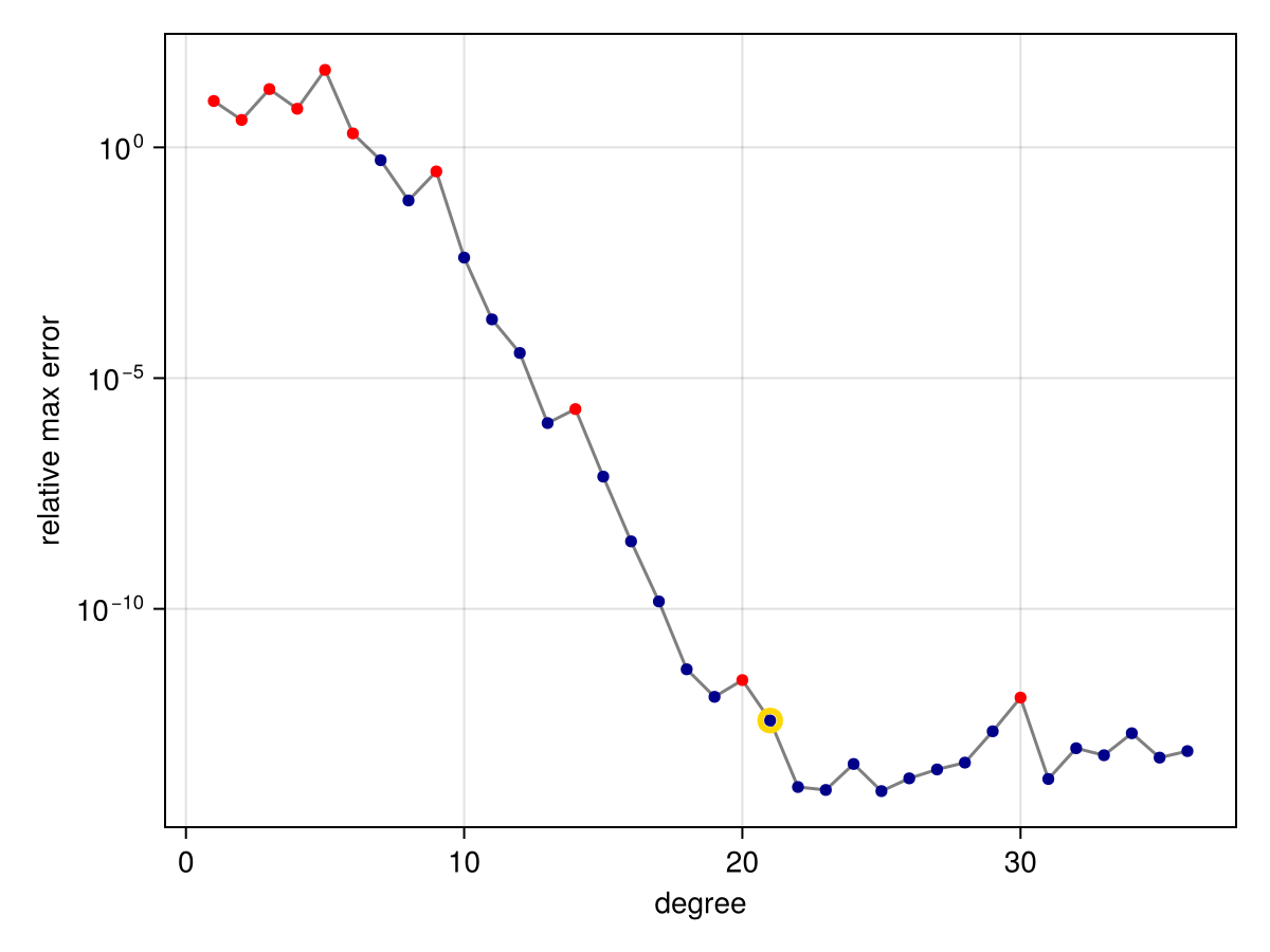

(The plots in this documentation are made using CairoMakie, but the same functions are made available for Plots.) In the plot above, the markers show the estimated max-norm error of the AAA rational approximant over the domain as a function of the denominator degree; each iteration adds one degree to both the numerator and denominator. The gold halo indicates the final approximation chosen by the algorithm.

The red dots in the convergence plot indicate that a genuine pole—that is, one with residue larger than machine precision—of the rational approximant lies in the approximation domain. We can verify this fact here by using rewind to recover the approximation from iteration 9:

julia> r9 = rewind(r, 9)
Barycentric{Float64, Float64} rational of type (9, 9) constructed on: Segment(-1.0,1.0)

julia> poles(r9)
9-element Vector{ComplexF64}:
 -0.8784983706895597 + 0.0im
  0.5359331936985986 + 0.3045387964361811im
  0.5359331936985987 - 0.3045387964361811im
  0.7487563504186071 + 0.17064861916801477im
  0.7487563504186072 - 0.17064861916801474im
  0.8823983414682102 - 0.12021541744242462im
  0.8823983414682102 + 0.12021541744242463im
  0.9721831701464687 - 0.07936858573736788im
  0.9721831701464687 + 0.0793685857373679im

What is going on near the "bad" pole? Let's isolate it and look at the point values of the approximation:

julia> x = first(filter(isreal, poles(r9)))
-0.8784983706895597 + 0.0im

julia> [r9(x), r9(x + 1e-6), r9(x + 1e-3)]
3-element Vector{ComplexF64}:
 -2.506614402665627e12 - 0.0im
    3609.3391058272623 + 0.0im
     4.657026725212222 + 0.0im

It's a genuine pole, but with a highly localized effect. At this stage of the iteration, AAA has not invested much resolution near this location:

julia> filter(<(-0.75), test_points(r9))
12-element Vector{Float64}:
 -1.0
 -0.9914930555555554
 -0.9829861111111111
 -0.9744791666666666
 -0.9659722222222222
 -0.9404513888888888
 -0.9149305555555556
 -0.8894097222222221
 -0.8638888888888889
 -0.8281597222222223
 -0.7924305555555555
 -0.7567013888888889

That's why the reported error is not very large. It's worth keeping in mind that the convergence plot shows the algorithm's estimate of the error, not the true error. Guarantees are hard to come by; no matter how carefully we told the algorithm to look within the interval, some cases would fall through the cracks. Fortunately, both the pole check and the overall error indicate that the approximation is not yet fully baked, and the iteration continues.

It is possible for the iteration to stagnate with bad poles if the original function has a singularity very close to the domain.

f = x -> tanh(500*(x - 1//4))
r = approximate(f, unit_interval)
convergenceplot(r)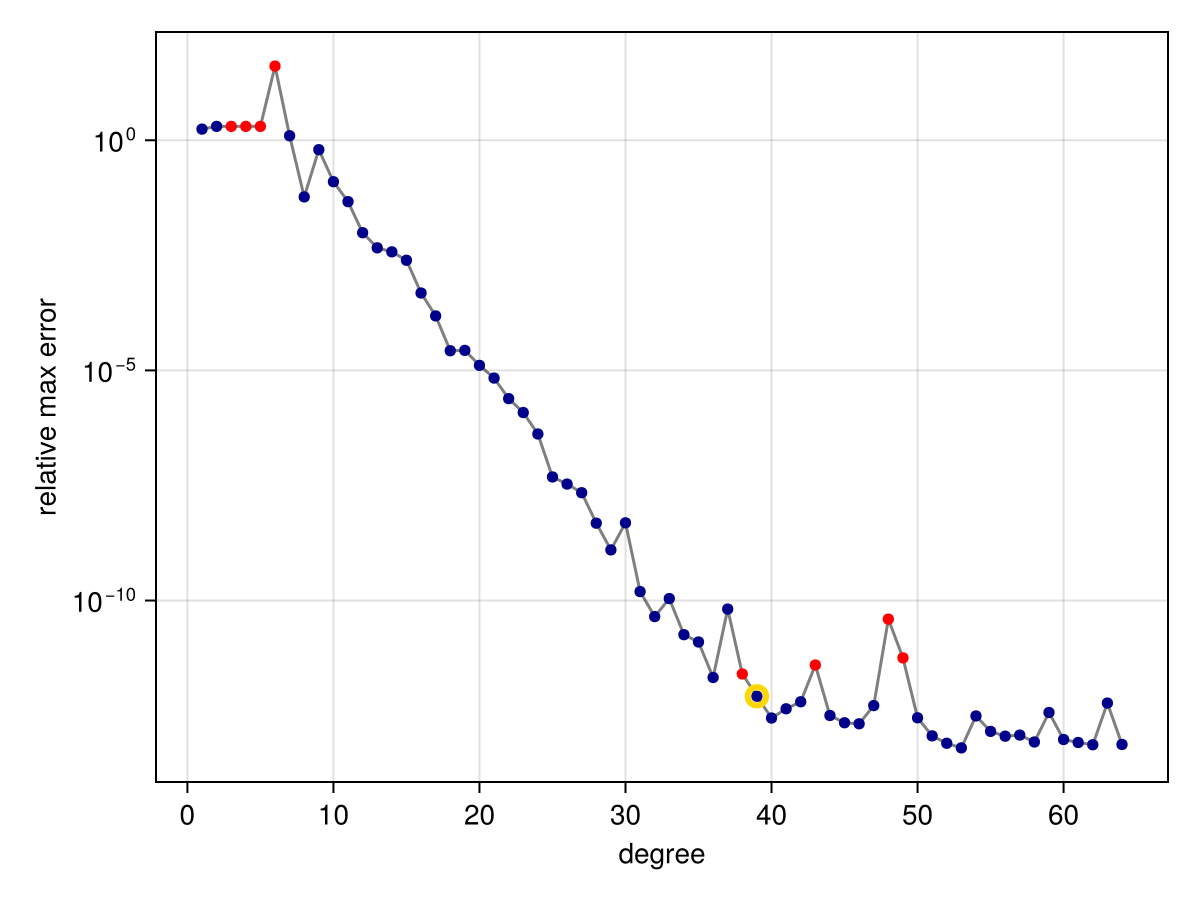

This effect is thought to be mainly due to roundoff and conditioning of the problem. In this case, if we use more accurate floating-point arithmetic, we can see that the AAA convergence continues steadily past the previous plateau. In the following, we apply Double64 arithmetic, having used exact rational numbers already in the definition of f:

using DoubleFloats, ComplexRegions
r = approximate(f, Segment{Double64}(-1, 1))
convergenceplot(r)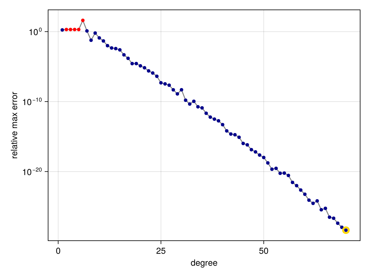

In the extreme case of a function with a singularity on the domain, the convergence can be substantially affected:

f = x -> abs(x - 1/8)
r = approximate(f, unit_interval)
convergenceplot(r)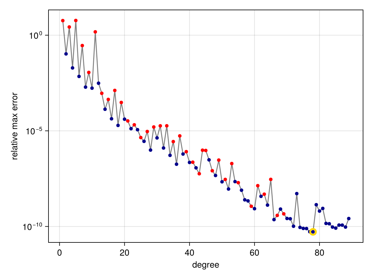

In such a case, we might get improvement by increasing the number of allowed consecutive failures via the stagnation keyword argument:

r = approximate(f, unit_interval, stagnation=50)
convergenceplot(r)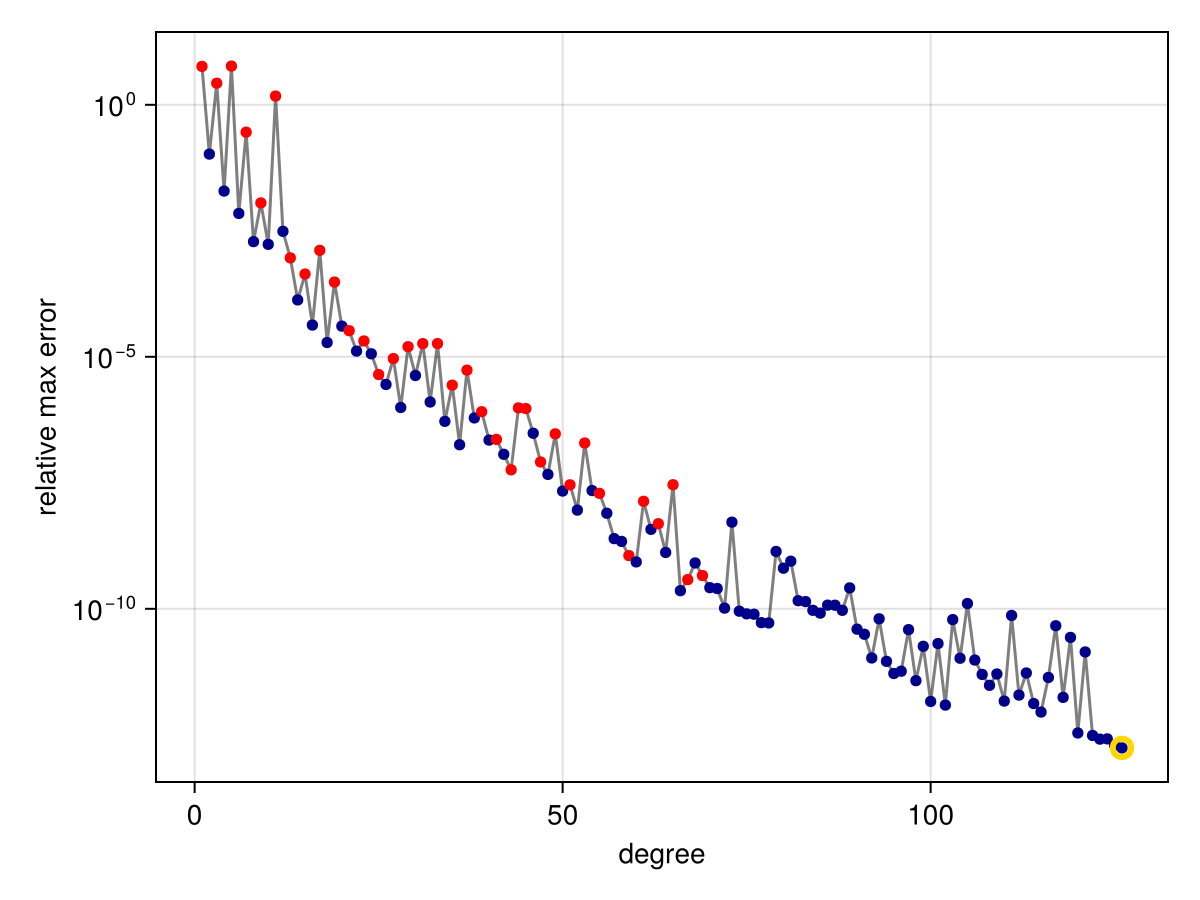

However, AAA is an $O(n^4)$ algorithm, so venturing into higher degrees can become costly.

Thiele continued fractions (TCF)

The TCF algorithm [5] is much newer than AAA and less thoroughly battle-tested, even though it's based on a continued fraction representation of rational functions that is over a century old. Like AAA, it uses iterative greedy node selection, and the effects of that ordering look good in experiments so far but are poorly understood theoretically. In TCF's favor are its $O(n^3)$ complexity requirement and an algorithmic simplicity that requires nothing more than basic arithmetic.

To try greedy TCF, use method=Thiele or method=TCF as an argument to approximate.

f = x -> cos(41x - 5) * exp(-10x^2)
r = approximate(f, unit_interval; method=TCF)
convergenceplot(r)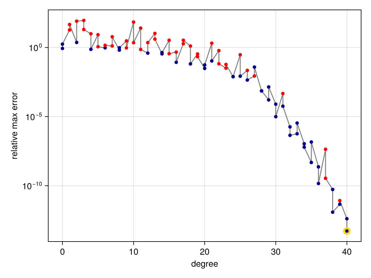

The $x$-axis of the convergence plot shows the degree of the denominator polynomial. Because the Thiele method alternates between interpolants of type $(n,n)$ and $(n+1,n)$, there are two dots in the plot for each degree.

Because TCF uses only addition, multiplication, and division, it is easy to use in extended precision arithmetic. Here, we use allowed=true to disable checking for poles, which requires solving an eigenvalue problem that is far more expensive than the iteration itself:

f = x -> atan(1e5*(x - 1//2))
domain = Segment{BigFloat}(-1, 1)
@elapsed r = approximate(f, domain; method=TCF, max_iter=400, allowed=true, stagnation=40)

28.444499173

convergenceplot(r)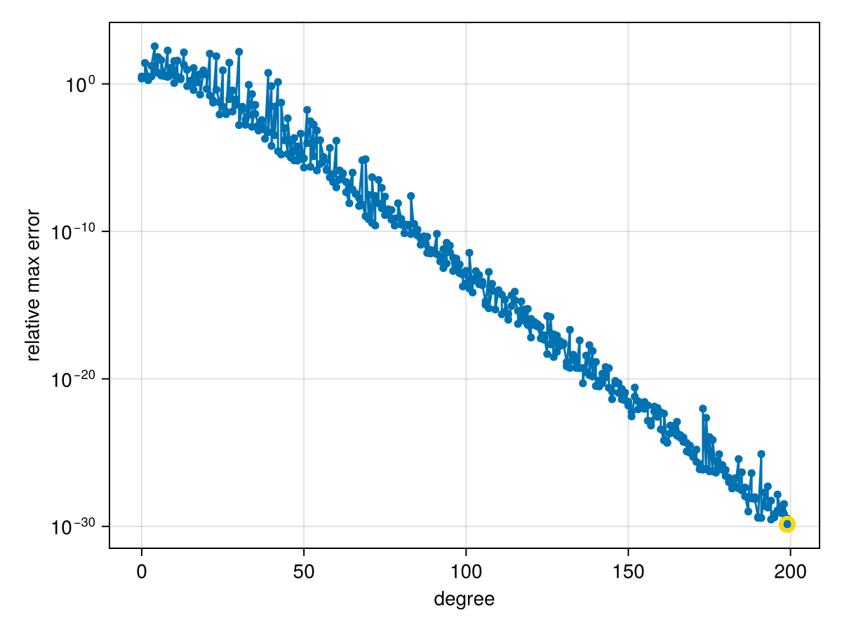

Prescribed poles

While AAA and TCF are nonlinear iterations, we can compute an approximation linearly if we prescribe the poles of the rational approximant. Specifically, given the poles ${\zeta }_1,\dots ,{\zeta }_n$, we can find a polynomial $p$ and residues $w_k$ such that

$$f(z)\approx p(z)+\sum _{k=1}^n\frac{w_k}{z-{\zeta }_k}.$$

When posed on a discrete set of test points, this is a linear least-squares problem. In order to represent the polynomial stably, an Arnoldi iteration is used to find a well-conditioned basis for the test points [6].

There is no iteration on the degree of the polynomial or rational parts of the approximant. In the continuum variant, though, the discretization of the boundary of the domain is refined iteratively until either the max-norm error is below a specified threshold or has stopped improving.

f = x -> tanh(x)
ζ = 1im * π * [-1/2, 1/2, -3/2, 3/2]
r = approximate(f, Segment(-2, 2), ζ)

PartialFractions{ComplexF64} rational function of type (6, 4) constructed on: Segment(-2.0,2.0)

max_err(r) = maximum(abs(r.original(x) - r(x)) for x in discretize(r.domain; ds=1/1000))
println("Max error: $(max_err(r))")

Max error: 1.9844602136220857e-5

To get greater accuracy, we can increase the degree of the polynomial part.

r = approximate(f, Segment(-2, 2), ζ; degree=20)
max_err(r)

3.663810827409843e-15

Note that the residues, which are all equal to 1 for the exact function, may not be reproduced by the rational approximation:

Pair.(residues(r)...)

4-element Vector{Pair{ComplexF64, ComplexF64}}:
 -0.0 - 1.5707963267948966im => 1.00000000487331 - 6.921820591153586e-11im
  0.0 + 1.5707963267948966im => 1.0000000048733098 + 6.921820146476337e-11im
   -0.0 - 4.71238898038469im => 0.009726848784147339 - 3.138033013139132e-11im
    0.0 + 4.71238898038469im => 0.009726848784147363 + 3.1380330237020535e-11im

Suppose now we approximate $|x|$ using AAA. We can extract the poles of the result.

r = approximate(abs, unit_interval, tol=1e-9)
ζ = poles(r)

60-element Vector{ComplexF64}:
 -0.0020262702905558456 - 0.18668690781706546im
 -0.0020262702905558456 + 0.18668690781706543im
 -0.0019064660623001434 + 0.11870564279657225im
 -0.0019064660623001432 - 0.11870564279657227im
 -0.0017487141593750775 - 0.2944600620064884im
 -0.0017487141593750775 + 0.2944600620064884im
  -0.001589739889065974 - 0.07535773488318508im
 -0.0015897398890659738 + 0.07535773488318509im
 -0.0011950044218827513 + 0.04762245012300538im
 -0.0011950044218827511 - 0.04762245012300538im
                        ⋮
  1.1337048082776984e-8 - 0.002325639919965619im
  4.7195492252636064e-6 - 0.004001550707133304im
  4.7195492252636064e-6 + 0.004001550707133304im
   7.936324196556495e-5 - 0.7840903991399022im
   7.936324196556497e-5 + 0.7840903991399021im
  0.0011275017553170534 - 1.4747962945471766im
  0.0011275017553170536 + 1.4747962945471769im
  0.0017816685246400035 + 4.70744746937112im
  0.0017816685246400037 - 4.70744746937112im

To what extent might these poles be suitable for a different function that has the same singularity?

s = approximate(x -> exp(abs(x)), unit_interval, ζ; degree=20)
max_err(r)

9.428162803422346e-10