Rational function approximation in Julia
Documentation for RationalFunctionApproximation.jl.
This package computes rational approximations of a function or data given in a domain in the complex plane (including real intervals).
A rational function is a ratio of two polynomials. Rational functions are capable of very high accuracy, usually requiring fewer degrees of freedom than polynomial approximations. They are an especially good choice for approximating functions with singularities near the domain of approximation. Rational functions have applications to finding singularities and roots, computing derivatives, continuation across boundaries, solving PDEs, and more; for a survey of applications, see [1]. For background on the algorithms in this package, see [2], [3] (or the related arXiv version [4]), [5], and [6].
Basic walkthrough
Here's a smooth, gentle function on the interval
using CairoMakie
CairoMakie.update_theme!(size = (600, 400), fontsize=11)
const shg = current_figure

f(x) = exp(cos(4x) - sin(3x))
lines(-1..1, f)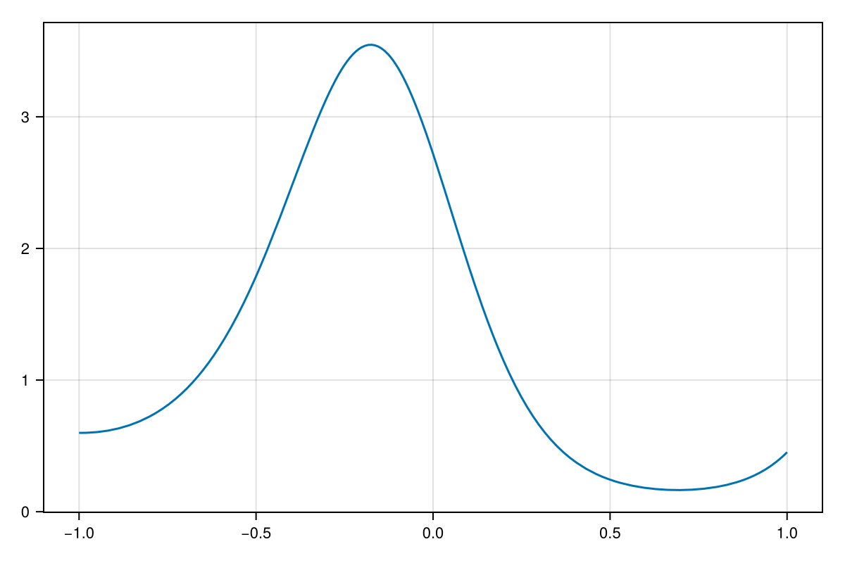
To create a rational function that approximates approximate function. By default, it uses the real interval
julia> using RationalFunctionApproximation

julia> r = approximate(f)
Thiele{Float64, Float64} rational of type (19, 18) constructed on: Segment(-1.0, 1.0)
  stopped by converged after 38 iterations with estimated error 2.298e-13
The result r is a type (19, 18) rational approximant that can be evaluated like a function:
julia> f(0.5) - r(0.5)
1.2295719997723609e-13
We see that this approximation is accurate to about 13 places over the interval:
z, err = check(r)
lines(z, err)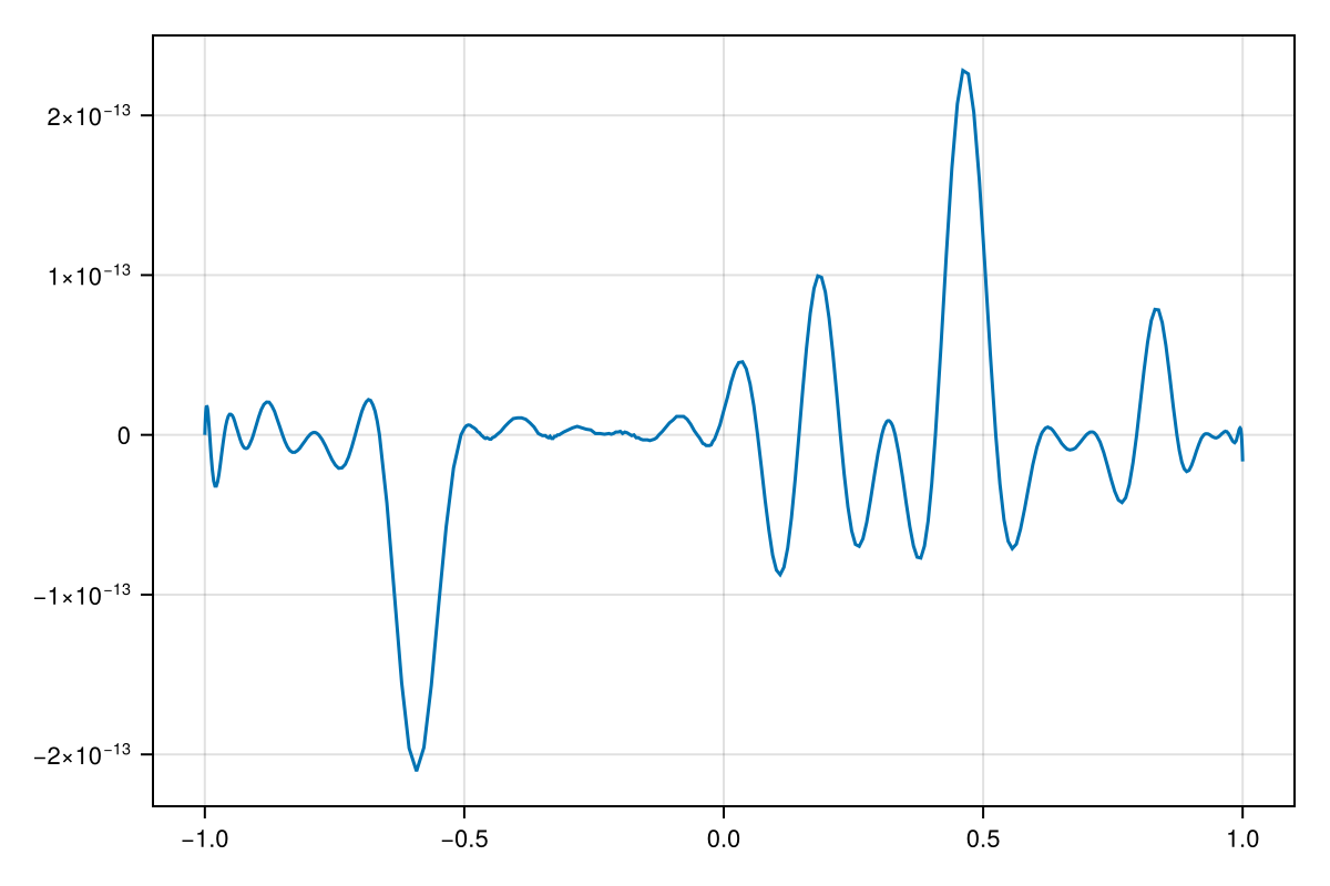
The rational approximant interpolates
x = nodes(r)
scatter!(x, 0*x, markersize = 8, color=:black)
shg()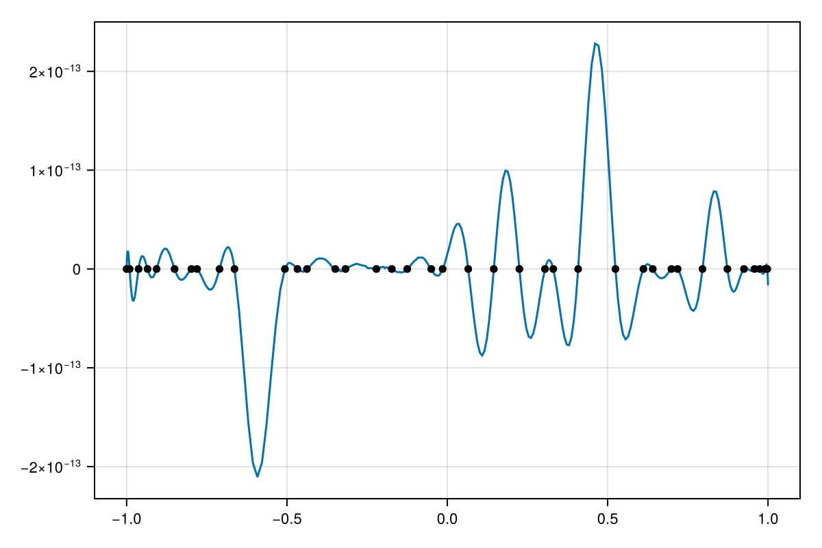
One important feature of a rational function is that it can have poles, or infinite value, at the roots of the denominator polynomial. In this case, the poles hint at where the function is most sharply peaked:
poleplot(r)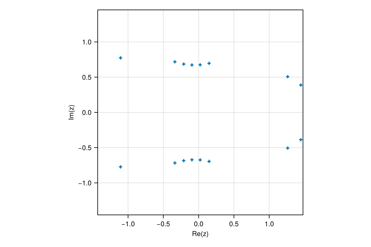
As another example, the sech function is smooth on the real axis but has poles on the imaginary axis at odd multiples of
r = approximate(sech, -4..4)
2 * poles(r) / π
10-element Vector{ComplexF64}:
-0.8386964483659707 - 6.966983928037078im
-0.8386964483659707 + 6.966983928037078im
-2.7093358498243922e-8 + 3.000001253761487im
-2.7093358498243915e-8 - 3.000001253761487im
9.846429674291083e-14 - 0.9999999999994963im
9.846429674291084e-14 + 0.9999999999994963im
3.1855517458318225e-5 + 4.993987578217663im
3.185551745831823e-5 - 4.993987578217662im
0.8396098221761168 + 6.968330829098956im
0.839609822176117 - 6.9683308290989565imWe can use the DomainColoring package to visualize the rational function in the complex plane. Color is used to show the phase angle of the value, while dark-to-bright cycles of lightness show powers of e in the magnitude. The poles stand out as locations of rapid change in both phase and magnitude.
using DomainColoring

domaincolor(r, 6; abs=true)
lines!(r.domain, linewidth=3, color=:white)
shg()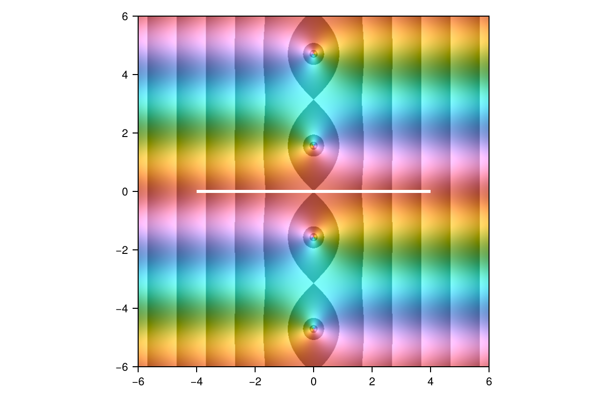
A meromorphic function such as sech has only those isolated poles as singularities, and getting those right is most of the battle. By contrast, the function
f(x) = log(x + 0.05im)
r = approximate(f)
domaincolor(r, 1.2; abs=true)
lines!(r.domain, linewidth=3, color=:white)
shg()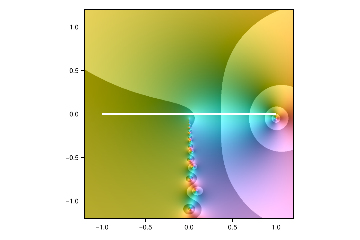
We close this quick introduction with approximation of
r = approximate(abs; tol=1e-12, stagnation=50)
convergenceplot(r)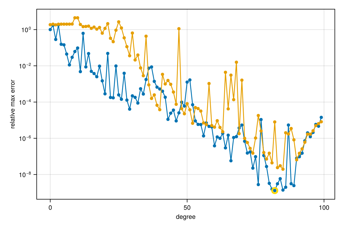
We find that the nodes of the approximant are also distributed (nearly) root-exponentially around the singularity:
z = filter(>(0), nodes(r))
scatter(sort(z), axis=(xlabel="index", ylabel="node location", xscale=sqrt, yscale=log10,))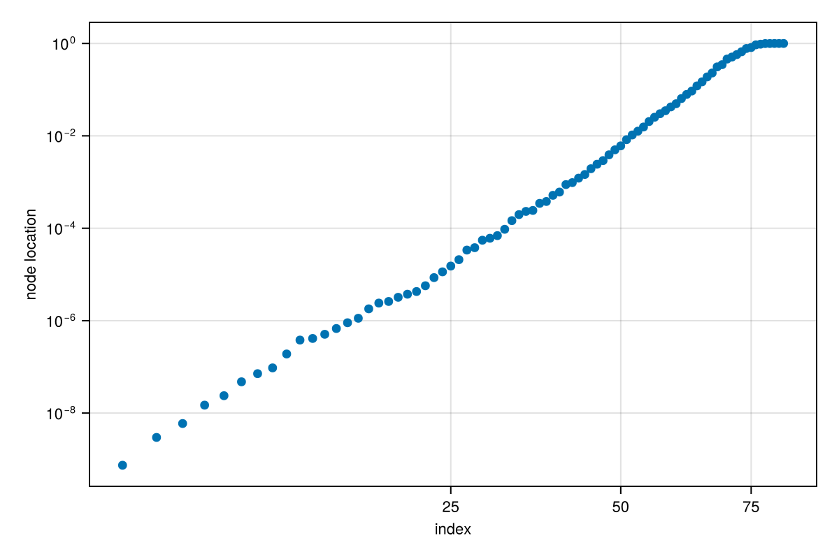
Feedback and contributions
If you encounter problems or want to make suggestions, feel free to file an issue on GitHub.
If you want to contribute to the package, please see the guidelines.
Contents
Installation describes the algorithms available for rational approximation.
Algorithms describes the algorithms available for rational approximation.
Approximation on domains shows how to approximate functions on different domains.
Discrete data shows how to approximate data given as points and values rather than as functions.
Minimax approximation explains the difference between the default approximation and minimax approximation.
Usage from Python shows how to use the package from Python.
Functions and types collects the documentation strings of the major package features.
References
Y. Nakatsukasa and L. N. Trefethen. Applications of AAA Rational Approximation. Acta Numerica 35, 459–601 (2026). Accessed on Jun 29, 2026.
Y. Nakatsukasa, O. Sète and L. N. Trefethen. The AAA Algorithm for Rational Approximation. SIAM Journal on Scientific Computing 40, A1494-A1522 (2018). Accessed on Jul 14, 2020.
T. A. Driscoll, Y. Nakatsukasa and L. N. Trefethen. AAA Rational Approximation on a Continuum. SIAM Journal on Scientific Computing 46, A929-A952 (2024). Accessed on May 15, 2025.
T. Driscoll, Y. Nakatsukasa and L. N. Trefethen. AAA Rational Approximation on a Continuum (2023). Accessed on Feb 26, 2024.
S. Costa and L. N. Trefethen. AAA-least Squares Rational Approximation and Solution of Laplace Problems. In: European Congress of Mathematics, 1 Edition, edited by A. Hujdurović, K. Kutnar, D. Marušič, Š. Miklavič, T. Pisanski and P. Šparl (EMS Press, 2023); pp. 511–534. Accessed on Oct 5, 2023.
O. Salazar Celis. Numerical Continued Fraction Interpolation. Ukrainian Mathematical Journal 76, 635–648 (2024). Accessed on Jan 28, 2025.
P. D. Brubeck, Y. Nakatsukasa and L. N. Trefethen. Vandermonde with Arnoldi. SIAM Review 63, 405–415 (2021). Accessed on Jun 5, 2025.
C. L. Lawson. Contributions to the Theory of Linear Least Maximum Approximations, Ph.D. Thesis, UCLA (Los Angeles, CA, 1961).